Quantifying Excitement

Using information theory to improve the ranking of NBA and WNBA games

Win probability graphs were my gateway drug to sports analytics, and my main motivation for building an NBA win probability model. The model has since been applied to a number of use cases, including when to foul, quantifying the importance of the four factors, and adding some analytic rigor to defining clutch play.

And with a win probability model in hand, you can also use it to craft statistics to evaluate a game and place it in context. How improbable was that comeback? Who had the most impressive clutch performance? How “tense” or uncertain was this game from start to finish?¹

And, how “exciting” was this game?

For that purpose, the win probability graphs at inpredictable.com feature an “excitement index” for each NBA and WNBA game. It’s a concept I borrowed from Brian Burke’s work at Advanced NFL Stats. As currently defined, the excitement index measures the cumulative, absolute change in win probability over the course of the game. Geometrically, think of it as the length of a win probability graph if it was a string and you pulled it taut.

This definition is easy to understand, and simple to deploy. But does it align what we, as human beings, would consider excitement?

Consider a play that takes a team’s win probability from 1% to 10%. Under the current definition of excitement, this is equally as exciting as a play that took a team from 41% win probability to 50%.

This is all subjective, but many would consider the 1st play to be more exciting, as it increases your chances of winning by tenfold, vaulting you from a nearly hopeless situation to one in which you have a fighting chance. A shift from 41% to 50% feels far less dislocating.

Information Theory to the Rescue

Are there better ways to measure excitement? It turns out there is - one with a more solid theoretical foundation and, most importantly, one that better aligns with objective measures of what actual human beings consider to be exciting games.

Rather than measure the absolute change in win probability, we can instead measure Kullback-Leibler Divergence. Put simply, KL-divergence measures the relative surprise between two separate probability distributions. In the parlance of information theory, it’s also known as relative entropy. If you don’t know what that means, don’t worry. Claude Shannon, inventor of information theory, borrowed the term on the advice of John Von Neumann, who told Shannon:

You should call it entropy, for two reasons. In the first place your uncertainty function has been used in statistical mechanics under that name, so it already has a name. In the second place, and more important, no one really knows what entropy really is, so in a debate you will always have the advantage

As with virtually all information theory formulas, KL-divergence involves logarithms, and is defined as follows:

The sum runs over all potential possibilities - for a basketball game, it’s just win or loss². P is considered the “true” probability distribution, and Q is the inferior, approximating distribution.

To calculate our new KL-inspired excitement index, we consider each play of the game as shifting us from the approximating probability Q to the new “true” probability P. We do this play by play, in order, and sum up a cumulative KL-divergence over the course of the game.

Returning to our 1%→10%, 41%→50% example, the KL-divergence of 1%→10% is 0.208, while the same calculation for 41%→50% yields just 0.024. Despite being the same additive change in win probability, KL-divergence finds a shift from 1% to 10% far more surprising by a factor of 10.

For binary probabilities, a KL-divergence of 1 is equivalent to finding out the outcome of a flipped coin. So, as we accumulate KL-divergence on a play by play basis, the resulting total tells us, in units of coin flips revealed, how much information, or surprise, was revealed by the game.

We’ll illustrate with one of the best games of the past decade: The Pacers’ late game comeback against the Knicks in the 2025 Eastern Conference Finals, culminating in an absurd, ballistically improbable overtime-forcing buzzer beater from Tyrese Haliburton:

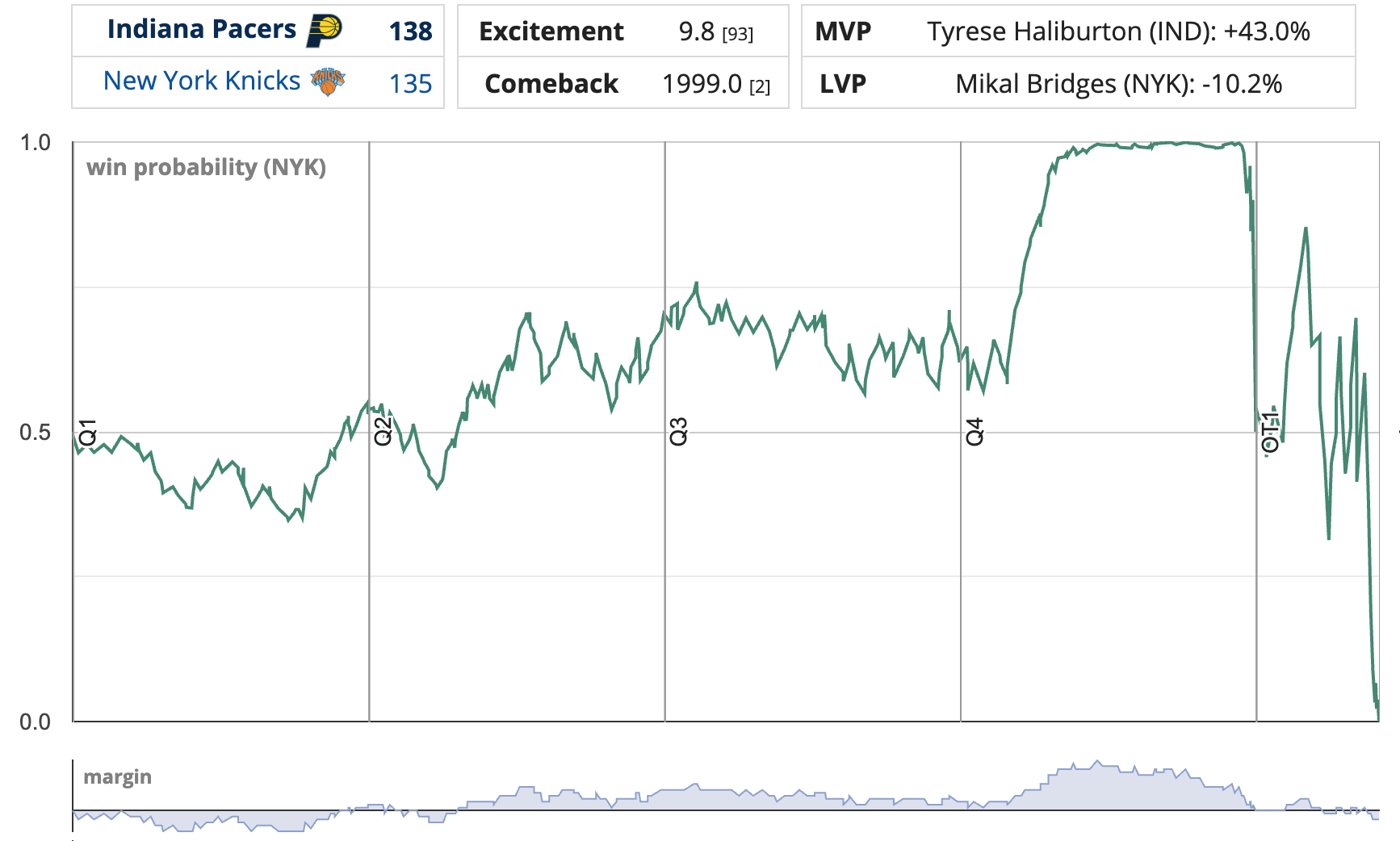
This game scores highly under either measure of excitement³, but a cumulative graph of both illustrates where KL-Divergence places more weight.

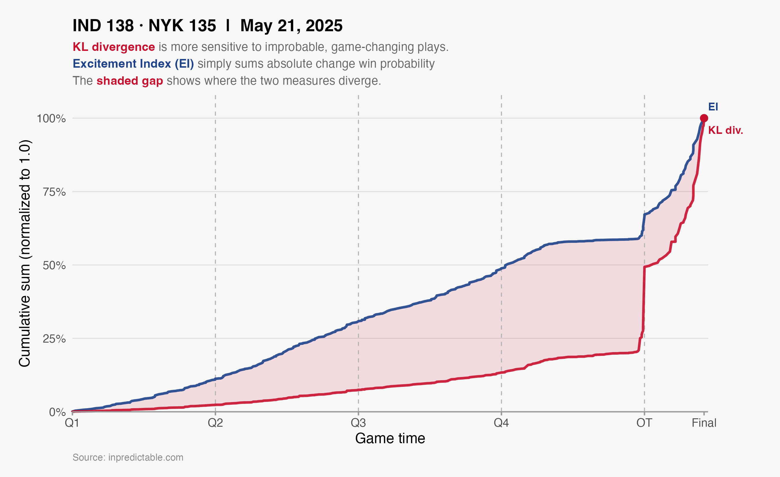
Haliburton’s game-tying long 2 improved the Pacers’ chances from 14% to 49%, an additive increase of 35%. To put that in context, let’s contrast that with an earlier two point shot from the 2nd quarter. With 3:20 left in Q2, Tyrese hit a turnaround jump shot that cut the Knicks lead from 6 to 4, and improved the Pacers’ win probability by 2.6% (from 36.4% to 39.0%). By our current excitement index measure, Haliburton’s buzzer beater was ~14 times more exciting than that 2nd quarter play.

How does KL-divergence assess the relative excitement of these two plays? For the buzzer beater, the KL-divergence is 0.501⁴. For the 2nd quarter play, that number is 0.002⁵.

So, by KL-divergence Haliburton’s iconic shot is 250 times more exciting than his 2nd quarter two pointer, much higher than what our current excitement index would say. We can see this in the chart above, with cumulative KL-divergence being far more responsive to late game plays, as compared to the current Excitement Index.

Another way in which KL-divergence better aligns with our own intuitive understanding of excitement is how it values large swings in win probability that occur as the result of a single play. Consider two potential scenarios:

• Scenario A (two plays): Play 1 takes the win probability from 0.50 to 0.60. Play 2 advances the win probability from 0.60 to 0.70

• Scenario B (one play): A single play takes the win probability from 0.50 to 0.70

Under the current definition of excitement index, Scenario A (+0.10 + 0.10) is scored identically to Scenario B (+0.20).

But KL-Divergence views Scenario B as more exciting:

• Scenario A KL-Divergence: 0.029 + 0.031 = 0.060

• Scenario B KL-Divergence: 0.119

That a single sudden lurch in win probability is more exciting than a steady IV drip of low impact plays certainly aligns with our intuition.

Comparison to Wikihoops User Ratings

I don’t know if anyone can quantify their own excitement to this level of precision, but KL-divergence definitely feels like it’s better attuned to what we subjectively think of as exciting.

And it turns out that we can support this with actual data. The creator of the fantastic NBA resource WikiHoops was kind enough to share data on how users of their site ranked every game from the 2024-25 NBA season.⁶

This gives us a crowd-sourced ranking of each game which we can then compare to both the existing Excitement Index as well as cumulative KL-Divergence.

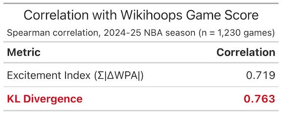
Both metrics correlate well with Wikihoops game score (a correlation of 1.0 would indicate identical ranking), but KL-Divergence has a stronger alignment.

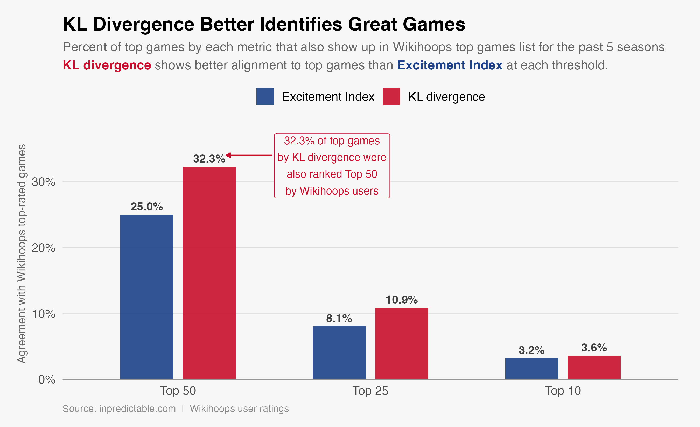
We can also measure how each metric aligns with the top games each season, as ranked by Wikihoops users. Whether by top 50, top 25, or top 10, KL-Divergence rankings have more overlap with Wikihoops user scores than the current version of Excitement Index

Next Steps

Having established KL-Divergence’s theoretical and practical bonafides, the next step is to deploy it as the new, improved version of Excitement Index on inpredictable for both the NBA and WNBA.

One mathematical caveat: The official metric will be defined as 2^[KL Divergence]. We don’t often think in logarithmic terms, so this converts the metric from “number of coin flips revealed” to “number of possibilities that were whittled down to one”. If you flip a coin 6 times, there are 64 potential outcomes, so a KL divergence of 6 is like revealing 1 outcome from a potential list of 64.

Defining excitement in this way also creates better numerical separation between the merely good games, and the instant classics. A score of 100 by this metric would place the game in the 99.9th percentile of exciting games.

1. When creating the Tension Index, I first employed a kludge-y, somewhat arbitrary way to define tension. However, in a later post I updated the definition to align with the information-theoretic concept of Shannon entropy What follows in this post is essentially doing the same for the excitement index.

2. This formula extends easily to games in which outcomes are not binary, such as a soccer match with separate probabilities of win, draw, or loss.

3. 9.8 for Excitement Index and 2.54 coin flips revealed for KL_divergence

4. 0.501 = 0.49 x log2(0.49/0.14) + 0.51 x log2(0.51/0.86)

5. 0.002 = 0.39 x log2(0.39/0.364) + 0.61 x log2(0.61/0.636)

6. Users can rate each game with a thumbs up or a thumbs down. Top games are those with the highest difference between thumbs up and thumbs down scores.